

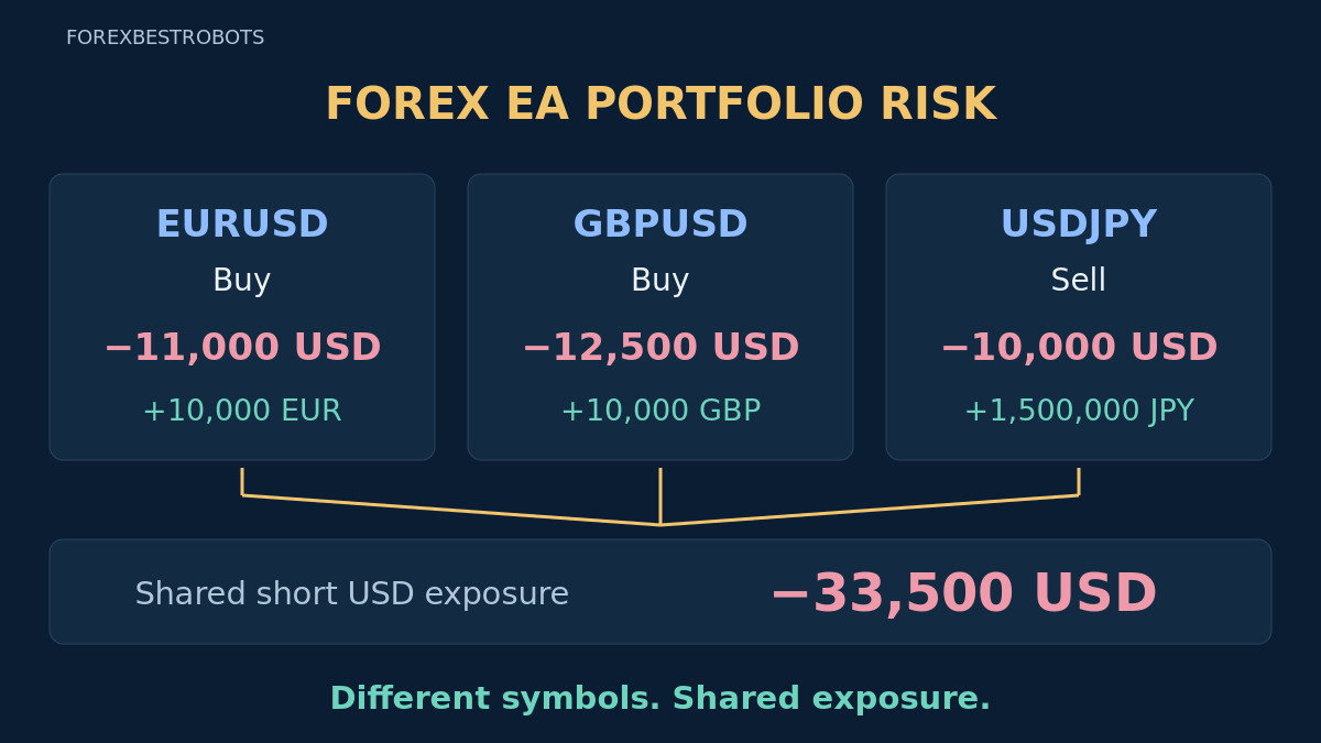
Running more EAs does not automatically spread risk. Different symbols can express the same currency view, and strategies with a low average correlation can still lose together. The useful question is what the whole account is exposed to at the same time.
Review currency direction, simultaneous positions, aligned equity changes and common stress scenarios together. The position example and the separate correlation example below are invented teaching cases. They do not establish a profitable portfolio or prescribe an allocation.
1. Define the whole portfolio before measuring it
Start with the evidence checks in the EA evaluation guide. Then list every EA, manual position and pending order within the review scope. Include accounts or terminals sharing the same capital or risk limit; separate accounts still need a common reporting currency and aligned valuations before their results can be combined.
- Positions: account, EA version, symbol, direction, volume, contract size and current mark.
- Future exposure: pending orders, grids, averaging rules and maximum permitted simultaneous positions.
- Data: common clock, account currency, cash flows, open P/L, costs and missing intervals.
- Dependencies: shared currencies, signals, sessions, broker, liquidity feed, VPS and execution constraints.
Attribute trades using deployment records and a checked Magic Number scope, without treating the identifier as proof by itself. Keep unknown exposure marked unknown. A missing position export is not a flat account, and an unfilled pending order is not current exposure but can become exposure later.
2. Translate each pair into currency directions
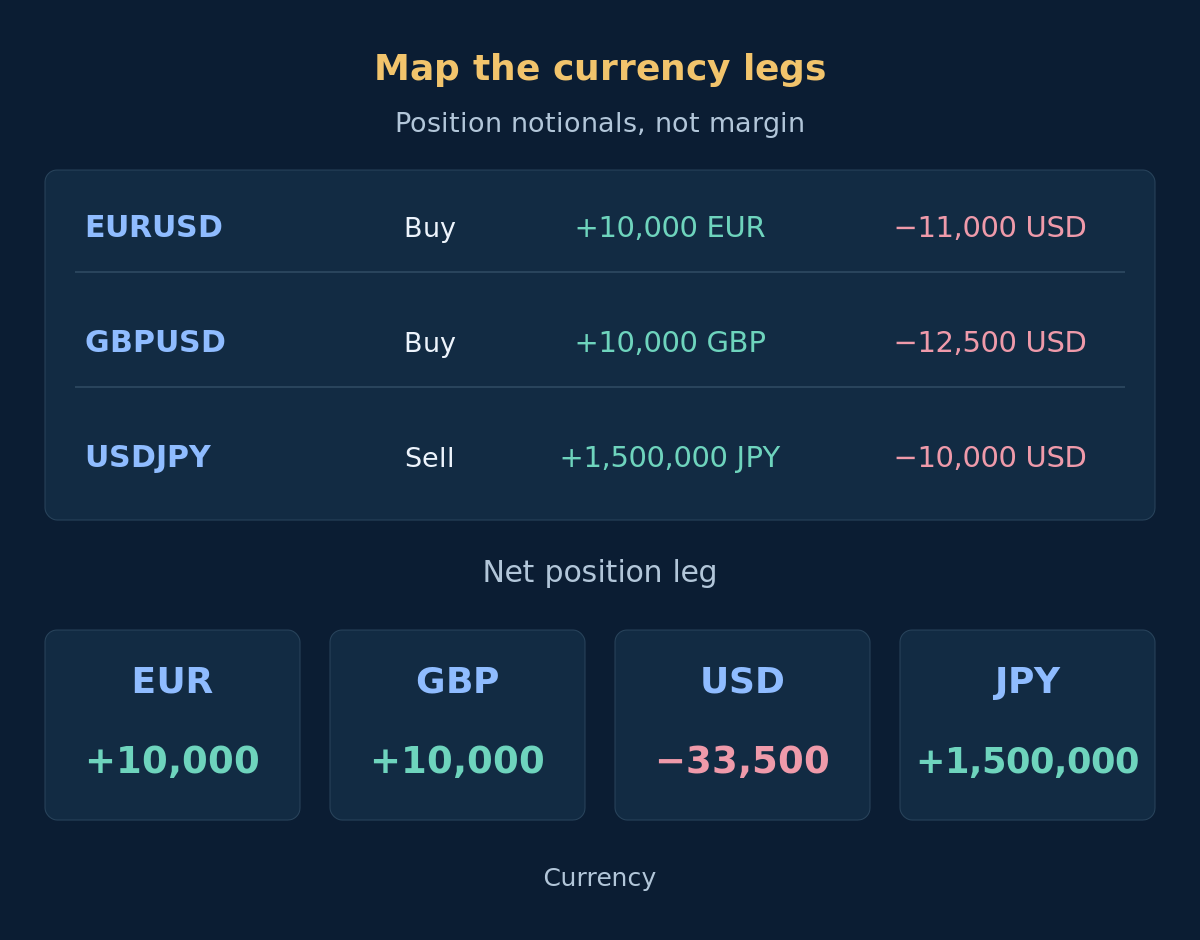
In the linear Forex model used here, buying a pair gives positive exposure to its base currency and negative exposure to its quote currency; selling reverses those directions. BUY EURUSD and SELL USDJPY both contain a short USD leg. Opposite order labels therefore do not necessarily offset the same risk.
Read the broker's actual contract specifications, including base/profit currency, contract size and account-currency conversion. Do not assume all symbols or cent accounts use identical units. The map below describes the positions' price exposure, not physical deliveries or cash loans. Keep account collateral and required margin separate from this map.
3. Calculate a frozen currency-exposure snapshot
Assume three invented linear Forex positions, each 0.10 lot with a contract size of 100,000 base-currency units per lot. Use the reference prices below, ignore costs for this first map, and keep position sizes fixed. Positive and negative signs indicate directional legs in their own currency units.
| System | Position | Lots | Reference price | Directional currency legs |
|---|---|---|---|---|
| EA-A | BUY EURUSD | 0.10 | 1.1000 | +10,000 EUR / −11,000 USD |
| EA-B | BUY GBPUSD | 0.10 | 1.2500 | +10,000 GBP / −12,500 USD |
| EA-C | SELL USDJPY | 0.10 | 150.00 | −10,000 USD / +1,500,000 JPY |
The USD legs add to −11,000 − 12,500 − 10,000 = −33,500 USD. The other net legs are +10,000 EUR, +10,000 GBP and +1,500,000 JPY. Do not add unlike currency units into one raw total. This snapshot reveals shared USD exposure; it is not the money deposited, margin used or a guaranteed loss for a particular percentage move.
4. Apply a coherent common shock
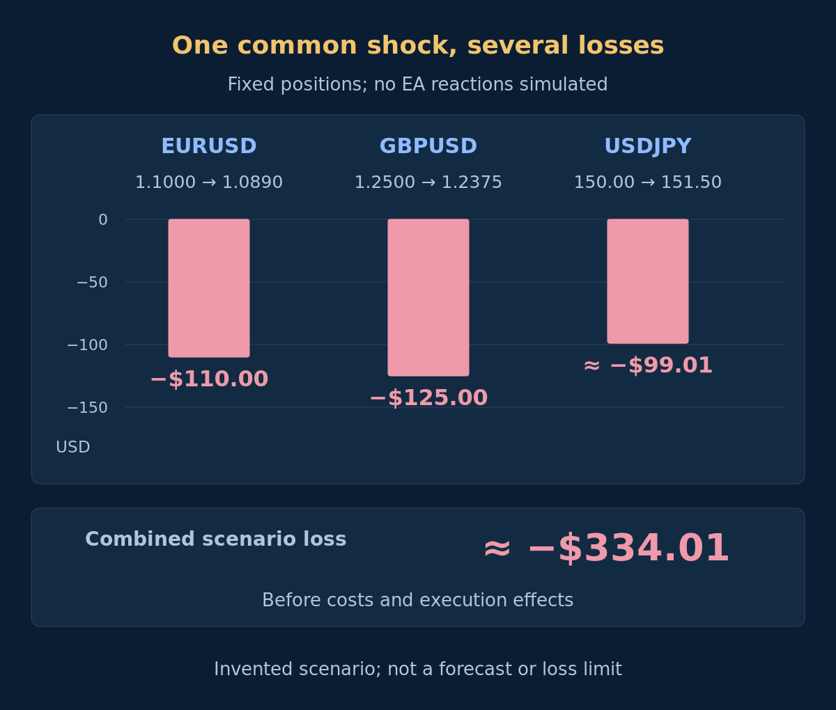
Keep those positions unchanged and revalue them at the invented prices below. EURUSD and GBPUSD each fall 1% from their reference, while USDJPY rises 1%. Use single, spread-free marks solely for this arithmetic; no actual Bid/Ask fills, fees, margin constraints or EA responses are simulated.
| Symbol | Reference | Shocked mark | Scenario P/L · USD |
|---|---|---|---|
| EURUSD | 1.1000 | 1.0890 | −$110.00 |
| GBPUSD | 1.2500 | 1.2375 | −$125.00 |
| USDJPY | 150.00 | 151.50 | ≈ −$99.01 |
All three lose despite different symbols and BUY/SELL labels. The combined loss is approximately $334.01, or 3.34% of illustrative $10,000 equity, before costs. These percentages describe the chosen scenario, not recommended risk. Actual spreads, gaps, currency conversion and changing positions can produce a different or larger loss; use the cost guide when extending the model.
Optional: reproduce the quote-currency conversion
EURUSD: 10,000 × (1.0890 − 1.1000) = −$110. GBPUSD: 10,000 × (1.2375 − 1.2500) = −$125. The USDJPY short loses 10,000 × (150.00 − 151.50) = −15,000 JPY; converting at the shocked mark gives −15,000 / 151.50 ≈ −$99.01. Sum the unrounded USD results: −110 − 125 − 15,000 / 151.50 ≈ −$334.01. Decimal points and thousands commas follow English numeric notation.
5. Align the data before calculating correlation
For actual evaluation, use matching intervals and a documented series that includes changes in open P/L, realized results and attributed costs. Reconcile cash flows and any unassigned account charges. Closed-ticket profit grouped by closing day can hide simultaneous floating losses. Specify whether you analyse returns on defined capital or fixed-base P/L contributions; changing position size can distort comparisons.
Use a common timestamp and overlapping sample dates. A genuine verified no-position interval may contribute zero; missing prices or an absent update must not silently become zero. Record the sampling frequency, number of observations and sizing changes. Pair-price correlation is not automatically EA-result correlation, because entries, direction, holding time and execution differ.
6. See how zero correlation can still allow a common loss
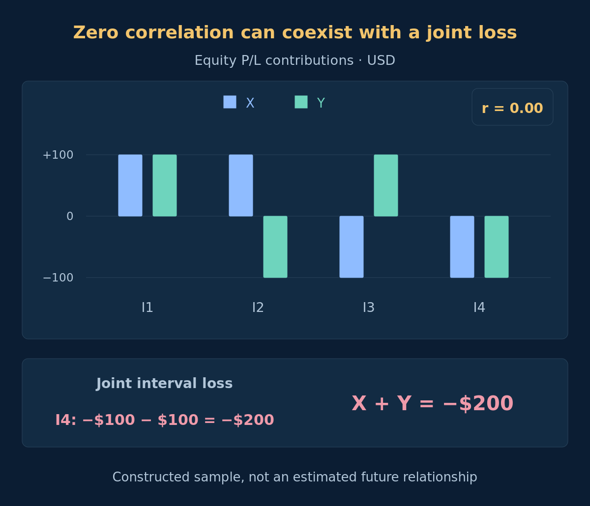
This separate constructed example uses four aligned interval equity-P/L contributions for systems X and Y, with fixed sizing and no cash flows or unassigned costs. It is unrelated to the three-position snapshot. The figures include realized and floating P/L changes; they are not returns on separately allocated accounts.
| Interval | X · USD | Y · USD | X + Y · USD |
|---|---|---|---|
| I1 | +$100 | +$100 | +$200 |
| I2 | +$100 | −$100 | $0 |
| I3 | −$100 | +$100 | $0 |
| I4 | −$100 | −$100 | −$200 |
Both sample means are zero. The cross-products cancel, so Pearson r = 0.00; yet at I4 both lose $100 and the account loses $200. Zero linear correlation does not imply independence or rule out simultaneous losses. Four deliberately constructed observations are enough to demonstrate that logic, not enough to estimate a durable relationship or justify a portfolio.
7. Rebuild combined equity instead of adding drawdowns
In the X/Y example, start a shared no-flow account at $10,000. After I1–I4, its equity is $10,200, $10,200, $10,200 and $10,000. The maximum observed account decline is $200 from a $10,200 peak, about 1.96%. This uses only the supplied marks; deeper intraperiod losses remain unknown.
Over the same marks, cumulative X contributions fall $200 from their own peak and Y contributions fall $100. Their sum is $300, not the account's $200 drawdown. Component peaks and declines need not align. Do not average or add published drawdown percentages. Reconstruct simultaneous, cash-flow-consistent equity in one currency; separately funded accounts require their actual capital and conversion history.
9. Compare adding an EA under fixed assumptions
Compare the existing portfolio with the proposed addition on the same dates, capital basis, exposure policy and cost model. Preserve all candidates and use later chronological validation rather than choosing the combination with the prettiest historical curve. Inspect the marginal change in currency legs, simultaneous losses, equity drawdown and margin usage, not only the added EA's standalone profit.
A static sum of standalone backtests may be invalid if shared margin, entry limits or execution cause trades to change. Replay the combined rules in time order and use backtesting checks, then controlled forward observation. State what cannot be reconstructed. Allocation sizes and account-level pause/resume rules need their own specification; this guide diagnoses exposure rather than choosing weights.
10. Keep a portfolio review sheet
A useful review should make the following questions answerable before increasing exposure. Set the review criteria in advance and retain missing-data flags and rejected candidates.
- Are all current positions and potential pending/grid exposure included?
- Are contract units, currency legs and conversion methods verified?
- Are equity changes, costs and cash flows aligned on the same clock?
- What happens when a common currency or execution shock hits the positions together?
- Does the joint-loss history support the interpretation of the correlation number?
- Can the combined equity and margin path be reproduced under the actual shared rules?
Document the snapshot date, configuration versions, sample period, attribution method, scenarios and unresolved limits. An incomplete exposure map is not evidence of diversification. Even a well-documented review cannot establish a future loss ceiling or guarantee that an added EA improves the portfolio.
11. Questions about EA portfolio risk
Do different Forex pairs guarantee diversification?
No. Their currency legs can overlap, and their strategies may react to the same event. Map direction and size together, then examine combined equity and common shocks.
Does zero correlation mean the EAs cannot lose together?
No. Our constructed X/Y sample has zero Pearson correlation and a simultaneous losing interval. Linear correlation alone neither proves independence nor describes every tail outcome.
Can I add the EAs' maximum drawdowns?
Not to obtain the actual portfolio drawdown. Different peaks, timing, cash flows and position constraints matter. Rebuild the common equity path; a sum can be a separately labeled stress assumption, not the observed combined statistic.
Is the currency-exposure map the same as required margin?
No. Directional notional describes position sensitivity. Margin is determined by the broker's contract and account rules and can change. Neither margin nor a stop order guarantees a maximum realized loss.
12. Sources and scope
The official MQL4 symbol-properties reference documents contract and currency fields; the NIST statistical glossary defines linear correlation; Investor.gov's diversification guide explains that diversification cannot guarantee protection from losses. They do not validate the invented portfolios or select allocation weights. Sources checked on 2026-10-18.
All positions, marks and interval results here are invented teaching inputs. The common-shock calculation and the separate X/Y dataset are different examples, not a backtest or verified performance. No future return, loss probability or suitable portfolio allocation is claimed.