

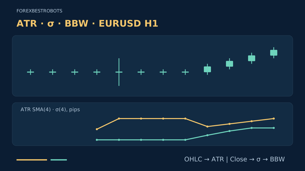
Two charts can look active for different reasons. Long wicks can increase a range measure without moving the closing prices, while orderly drift can spread closes around their average. A useful volatility comparison starts with the question each indicator answers, rather than treating every rising line as the same evidence.
This second guide compares measurements and their roles. It does not supply a breakout system, entry threshold or position-sizing rule. The ATR construction guide covers True Range, smoothing and pip conversion in detail. Here, one common data set makes the differences between ATR, close-price standard deviation and Bollinger BandWidth visible.
1. Match the indicator to a specific question
Use ATR to summarize recent True Range, including the relationship between the current high/low and the previous close. Use standard deviation to describe how selected price observations are dispersed around their mean. Use BandWidth to express a Bollinger envelope's width relative to its middle line.
These are descriptions, not interchangeable forecasts. A larger reading does not choose BUY or SELL, prove a reversal, set a maximum future range or establish a profitable trade. All three depend on the symbol, timeframe, data and calculation choices.
Write down whether you need a price-distance context, dispersion of closes, or relative band contraction. Assign one role to each retained input. Adding more volatility panels does not automatically add information.
2. Keep the ATR definition explicit
For valid Bid candles, TR = max(H, Cprev) − min(L, Cprev). This guide uses ATR_SMA(t) = Σ TR(t−j) / n, j = 0…n−1. Its rolling arithmetic mean is chosen to align the sample windows for teaching, not because every platform uses it.
A Wilder average or another initialization can produce different values. Record that choice before comparing indicators. ATR retains high/low information that a calculation using only closes cannot see; it does not describe the order of ticks within a candle or the price movement still to come.
3. Define standard deviation of prices, not returns
Let M be the arithmetic mean of the latest n completed closes: M(t) = Σ C(t−j) / n, j = 0…n−1. Define σ(t) = sqrt(Σ (C(t−j) − M(t))² / n), j = 0…n−1. Every close in that window is compared with the same current-window mean.
The divisor here is n, the population convention for the selected window, rather than the sample divisor n−1. Changing the divisor, applied price, weighting or mean changes the specification. Standard deviation has price units; divide by the documented pip size if you want pips.
This is dispersion of price levels. It is not the standard deviation of percentage or log returns, and it is not annualized realized volatility. A steady directional drift can spread closes around their mean even when the step between consecutive closes is constant. Do not label that automatically as erratic trading.
4. Derive BandWidth from the same bands
For this example, use U = M + k × σ and L = M − k × σ, with an SMA middle line and the same close-price σ. With positive M, define BBW_pct = 100 × (U − L) / M. This guide always reports percentage units, not the unmultiplied ratio.
Algebra gives BBW_pct = 200 × k × σ / M. With k = 2, the full band distance is 4 × σ. An implementation using an EMA center, different weighting or another source is a different construction and must be matched before comparison.
BandWidth measures width, not where price sits inside the bands. The distinct position measure %b = (Close − L) / (U − L) is undefined when the band distance is zero. Neither a band touch nor a narrow width supplies a trade direction or a calibrated probability of what happens next.
5. Reproduce the common synthetic example
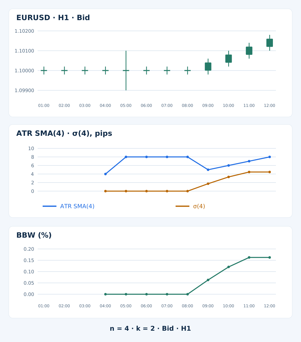
The table contains invented EURUSD H1 Bid candles labeled by closing time on one assumed server clock. The preceding 00:00 close is 1.10000. All lookbacks use n = 4; bands use k = 2. These short settings expose the arithmetic and are not recommended trading parameters. One pip is 0.00010.
| H1 close time | Bid open | Bid high | Bid low | Bid close | TR, pips | ATR SMA(4), pips | σ(4), pips | BBW, % |
|---|---|---|---|---|---|---|---|---|
01:00 | 1.10000 | 1.10020 | 1.09980 | 1.10000 | 4 | — | — | — |
02:00 | 1.10000 | 1.10020 | 1.09980 | 1.10000 | 4 | — | — | — |
03:00 | 1.10000 | 1.10020 | 1.09980 | 1.10000 | 4 | — | — | — |
04:00 | 1.10000 | 1.10020 | 1.09980 | 1.10000 | 4 | 4.000000 | 0.000000 | 0.000000 |
05:00 | 1.10000 | 1.10100 | 1.09900 | 1.10000 | 20 | 8.000000 | 0.000000 | 0.000000 |
06:00 | 1.10000 | 1.10020 | 1.09980 | 1.10000 | 4 | 8.000000 | 0.000000 | 0.000000 |
07:00 | 1.10000 | 1.10020 | 1.09980 | 1.10000 | 4 | 8.000000 | 0.000000 | 0.000000 |
08:00 | 1.10000 | 1.10020 | 1.09980 | 1.10000 | 4 | 8.000000 | 0.000000 | 0.000000 |
09:00 | 1.10000 | 1.10060 | 1.09980 | 1.10040 | 8 | 5.000000 | 1.732051 | 0.062978 |
10:00 | 1.10040 | 1.10100 | 1.10020 | 1.10080 | 8 | 6.000000 | 3.316625 | 0.120572 |
11:00 | 1.10080 | 1.10140 | 1.10060 | 1.10120 | 8 | 7.000000 | 4.472136 | 0.162534 |
12:00 | 1.10120 | 1.10180 | 1.10100 | 1.10160 | 8 | 8.000000 | 4.472136 | 0.162475 |
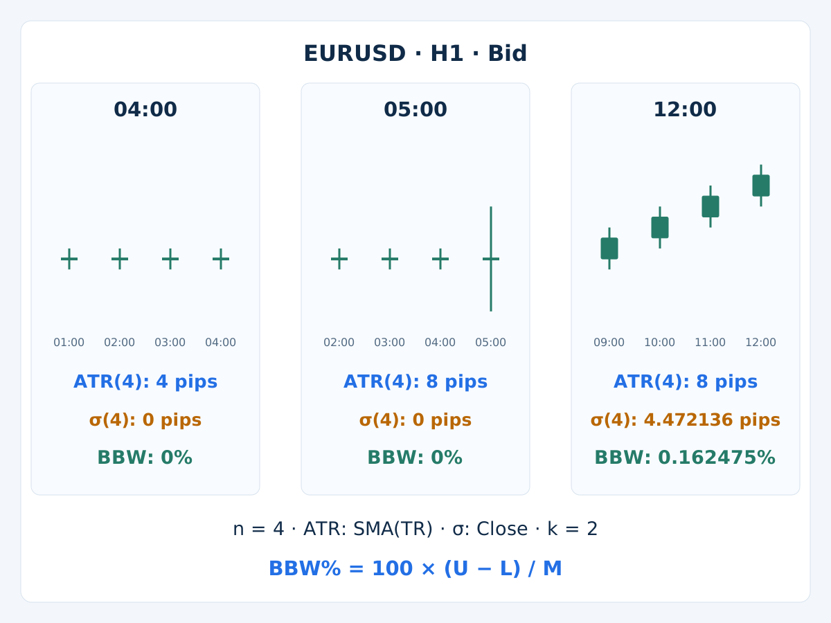
The first complete window ends at 04:00. Its closes all equal 1.10000, so σ and BBW are zero, while ATR is 4 pips. These are available measurements, not missing values. Earlier average and dispersion entries are unavailable. Displayed results are rounded to 6 decimals; calculations retain full precision.
At 05:00, the high and low widen while the close stays unchanged. TR is 20 pips, and ATR = (4 + 4 + 4 + 20) / 4 = 8 pips. The latest closes still match, so close-price σ and BBW remain zero. “Zero dispersion of closes” clearly does not mean “no intrabar movement.”
At 12:00, ATR is also 8 pips, but the latest closes differ. M is 1.10100; their offsets are −6, −2, 2, 6 pips. Thus σ = sqrt((36 + 4 + 4 + 36) / 4) = sqrt(20) pips, displayed as 4.472136. The full band distance is 17.888544 pips and BBW is 0.162475%. No order, fill or trading return is simulated.
6. Explain the disagreement before changing a rule
The wick example changes high/low ranges without changing closes. The later drift changes close dispersion. Equal ATR values can therefore coexist with different σ and BBW values. That is useful information about the definitions, not evidence that one indicator is broken or universally superior.
A falling rolling average can also reflect a large old observation leaving its window. At 09:00, the wide-wick TR has left our ATR window. More generally, changing the lookback or smoothing changes responsiveness and memory. Do not rank indicators by which line reacts fastest in one selected example.
7. Avoid counting the same dispersion twice
With the same M, σ and fixed band multiplier, BBW is an algebraic transformation of normalized σ. In particular, BBW_pct = 4 × (100 × σ / M) for the stated bands. Requiring both to rise does not provide two independent confirmations of volatility.
ATR uses additional OHLC information, but it still shares price data with the close-based measures; statistical independence is not implied. Prefer an explicit role for each input and test whether the added rule contributes anything. The indicator-combination guide explains how to separate complementary roles from repeated votes.
8. Normalize deliberately and preserve units
Raw ATR and σ are price distances. Here we can express ATR as 100 × ATR / Close, whereas BBW divides its full band distance by M. At 12:00, the ATR percentage is 0.072622% and BBW is 0.162475%. They have different numerators and denominators; a larger number does not make one a stronger signal.
Multiplying every price by the same positive constant multiplies raw distances but leaves these normalized ratios unchanged. That removes a price-scale effect, not differences in liquidity, session, timeframe, contract size or money risk. Do not transfer a pip convention or a percentage threshold between instruments without a fresh specification.
9. Define “low” relative to earlier observations
A BBW value is not intrinsically narrow across every pair and timeframe. Choose the historical reference, lookback, tie rule and warm-up requirements in advance. Compare only with observations already available at the decision time; a full-chart minimum or percentile can introduce future information.
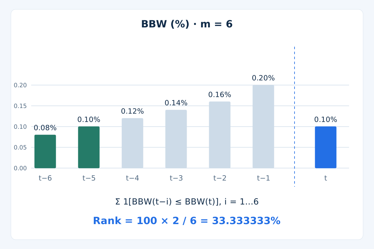
For a separate teaching example, let the previous six completed BBW readings be 0.08, 0.10, 0.12, 0.14, 0.16, 0.20 percent, and the current reading 0.10%. Define Rank = 100 × count(previous BBW ≤ current BBW) / m. Excluding the current reading from the reference set gives 100 × 2 / 6 = 33.333333%. This is a historical rank, not the probability of a breakout.
Ties matter: replacing “less than or equal” with “less than” changes that result. With an inclusive rule, an all-equal reference set gives rank 100%, so this rank is not a universal flat-market detector. Define and test the actual contraction rule separately. The existing Bollinger squeeze strategy covers a distinct price-confirmation framework; it is not supplied by the rank alone.
10. Align the platform inputs and observation time
In MT4, iStdDev(_Symbol, PERIOD_H1, 4, 0, MODE_SMA, PRICE_CLOSE, 1) explicitly names the method, source and closed-bar buffer shift. For bands, iBands(_Symbol, PERIOD_H1, 4, 2, 0, PRICE_CLOSE, MODE_UPPER, 1) selects the upper line. Read MODE_MAIN and MODE_LOWER with matching arguments to derive width. A line's chart displacement and its buffer shift are different parameters.
Record the exact broker symbol, quote side, timeframe, source, period, weighting, deviation multiplier, history and indicator version. Our ATR is explicitly a rolling SMA; do not assume a terminal's ATR matches it. Reconstruct the same candles and compare unrounded completed-bar values. This article does not claim to have verified a live terminal's output.
Immediately after 12:00 and once the data are ready, the candle that closed at 12:00 opened at 11:00 and is shift 1; the 12:00–13:00 candle is still forming at shift 0. Store the opening timestamp, not just a changing shift number. Different server boundaries or higher-timeframe bars require their own alignment.
11. Validate the measurement before judging a method
Require valid OHLC and enough contiguous observations; our ATR also needs a known preceding close. Do not fill missing data with zero or silently bridge an unexpected hole. Genuine zero σ or BBW can be valid, while a zero or nonpositive divisor must be rejected. Missing history and an uninitialized indicator are not evidence of low volatility.
These Bid-based measurements do not price an executable trade. Spread, commission, financing, slippage, volume and correlated exposure remain separate. The trading-cost guide and risk-management guide explain why neither a low normalized reading nor a multiple of an indicator is a complete risk model.
Reproduce constant closes with wicks, directional drift, outliers leaving a window, ties, zeros and missing history. Replay one completed bar at a time; later candles must not alter earlier results under unchanged data and initialization. If a measurement becomes a rule, preserve tried variants and later evaluation data, then forward-test. The MT4 backtesting guide covers the wider process. No indicator comparison proves a trading edge.
12. Questions about volatility comparisons
Which is best: ATR, standard deviation or BandWidth?
There is no universal winner. ATR summarizes True Range, standard deviation describes the selected prices' dispersion, and BandWidth normalizes a band distance. Choose the measurement that fits a defined question, then evaluate any trading rule separately.
Can σ be zero while ATR is positive?
Yes. Identical closing prices can coexist with high and low prices moving within each candle. Close-price dispersion and band width can be zero while True Range and its average remain positive. Check data readiness before interpreting zeros.
Are σ and BandWidth independent confirmations?
Not when they use the same closes, mean, dispersion convention and fixed multiplier. BandWidth is then a scaled form of normalized σ. Different labels do not make the underlying information independent.
Do two standard deviations guarantee a price-containment probability?
No. The construction does not establish normal, independent observations or a calibrated forecast. Do not attach a universal coverage probability to the bands or treat a band touch as an automatic reversal signal.
Is BBW of 0.10% always low?
No. Its meaning depends on the instrument, timeframe, settings and past reference. A historical rank also depends on its lookback and handling of ties. Neither the raw reading nor its rank guarantees that expansion is due.
Why do my platform readings disagree with this table?
Match the synthetic input candles first, then check the exact algorithm, divisor, source, window, shift, seed or warm-up, quote side and units. The example is explicitly specified arithmetic, not a verified reproduction of every platform implementation.
13. Technical reference and scope
John Bollinger's official rules explain the construction of traditional bands, normalized BandWidth and the limits of statistical assumptions. This guide states its own formulas, population divisor, data and timing so the comparisons can be reproduced without assuming that every implementation is identical.
Forex and leveraged trading involve substantial risk. This guide is educational, not investment advice. Past or simulated results do not guarantee future performance.