

A band touch describes relative location. A narrow band describes dispersion in a chosen window. Neither observation supplies an order by itself. This guide rebuilds Bollinger Bands from declared closes, separates position from width and shows how the rolling window changes what the chart means.
1. Name the three bands and the question they answer
Call the middle band M, the upper band U and the lower band L. Traditional Bollinger Bands place outer curves a chosen number of standard deviations from a simple moving average. They describe high and low relative to that calculation, rather than absolute cheapness or expensiveness.
The bands use historical prices, including the current observation when its value is calculated. An upper touch is not an automatic SELL, and a lower touch is not an automatic BUY. The original examples below explain indicator construction and reading; they do not report trading performance.
2. Fix the 20/2 inputs before comparing charts
Our reference is 20 / 2: twenty observations for both the simple mean and dispersion, with a two-standard-deviation multiplier on each side. The applied price is Close. On H1, twenty periods mean twenty bars, not twenty calendar days. Use an undisplaced display and record the actual symbol and price feed.
The multiplier is neither a percentage nor a probability. Two standard deviations do not establish that a future price has a 95% chance of remaining inside the bands. Rolling, overlapping market observations do not provide that distributional guarantee. Defaults are starting specifications, not evidence of profitable settings.
3. Calculate population dispersion from the same window
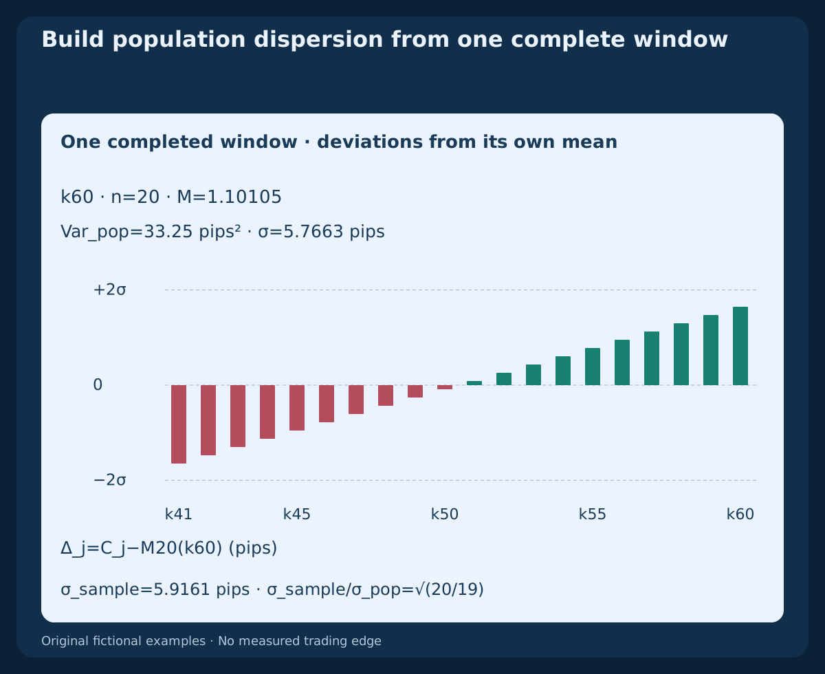
For the n closes ending at k, use M(k)=ΣC_j/n, Var_pop(k)=Σ(C_j−M(k))²/n and σ(k)=√Var_pop(k). Every deviation in that window is measured against its same current window mean. With zero-based indexing, the twenty-bar reference first exists at k19; earlier rows are unavailable.
Dividing by n−1 instead gives sample variance and different outer bands. For the same twenty closes, σ_sample=σ_pop×√(20/19). The fixture retains that comparison separately but uses population dispersion for its bands. A constant complete window has valid σ=0; this is different from insufficient history.
4. Read %B as location, including outside the bands
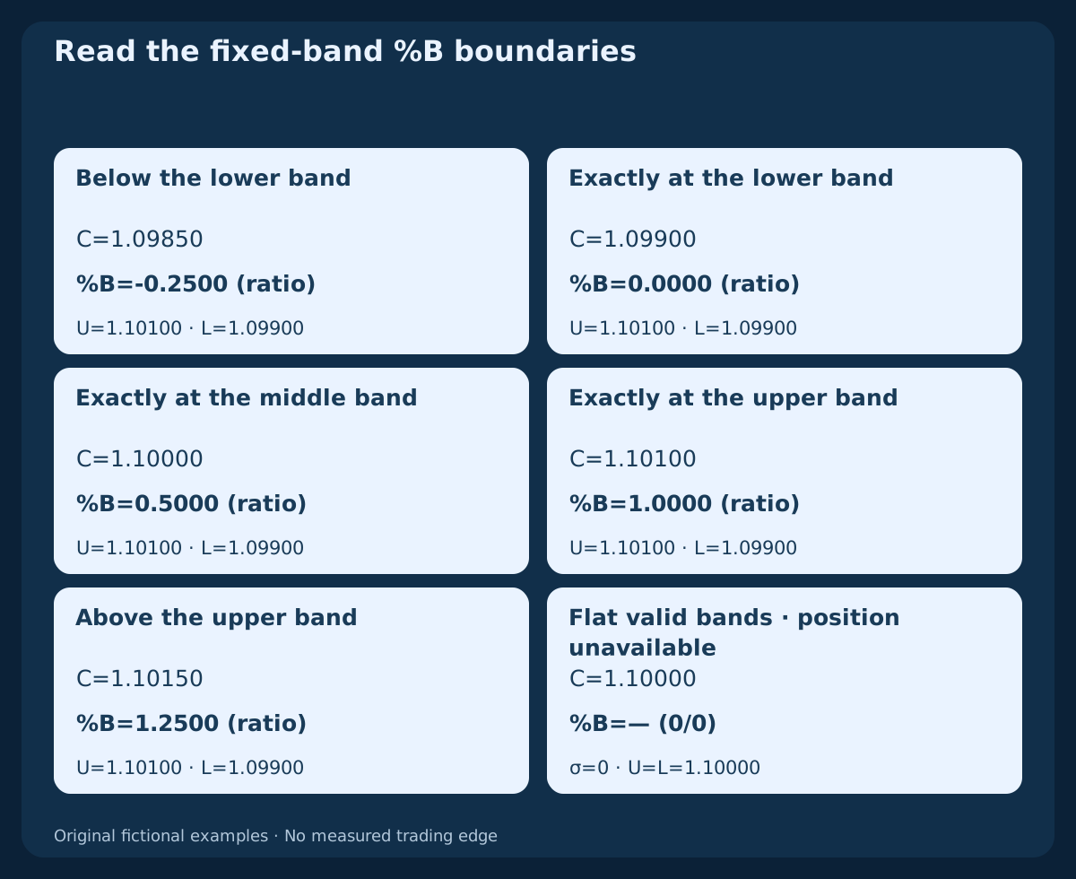
Define %B(k)=(C(k)−L(k))/(U(k)−L(k)). With symmetric nonzero bands, 0, 0.5 and 1 locate the lower, middle and upper band respectively. Values %B<0 and %B>1 are permitted: price is outside, not a calculation error. The independent fixed-band CSV makes these boundaries explicit.
We publish the ratio scale; some displays multiply it by one hundred. State the scale instead of inferring it from the percent sign in the name. When U=L, the location expression becomes 0/0 for our flat window and remains unavailable. We do not silently substitute a neutral value. Other implementations need their own documented fallback policy.
5. Keep raw width, normalized width and percent units distinct
Let W=U−L, BW_ratio=W/M and BW_pct=100×BW_ratio. This reference requires M>0 for normalized width. At the constructed alternating endpoint, BW_ratio≈0.00036298 is the same width as BW_pct≈0.036298%. A factor-of-one-hundred display difference is not different volatility.
With a positive middle and flat bands, BW_pct=0 is valid even though %B is unavailable. A zero or nonpositive middle is outside this positive-Forex normalization convention. Also, %BandWidth may name a separate normalization within a historical width range; it must not be assumed to mean merely multiplying raw width by one hundred. Inspect the formula.
6. Separate equal position from equal pip distance
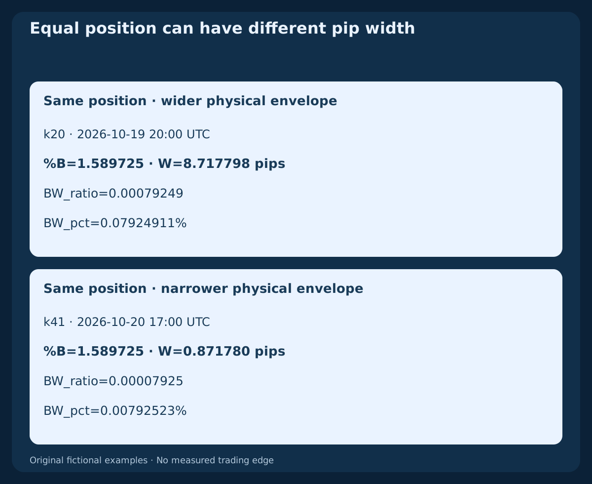
The first outlier at k20 and the first rise after the reset at k41 both have %B≈1.589725. Their full outer-band widths are W≈8.717798 pips and W≈0.871780 pips. For EURUSD this example declares 1 pip=0.0001. The position ratio agrees while the physical width differs tenfold.
Equal %B therefore does not imply equal stop distance, spread burden, risk or lot size. BandWidth divides width by the middle price; it is not ATR, a return-volatility estimate or a universal threshold across pairs and sessions. Preserve the price, pip and ratio units when comparing a calculation with execution costs.
7. Distinguish a state from a fresh completed crossing
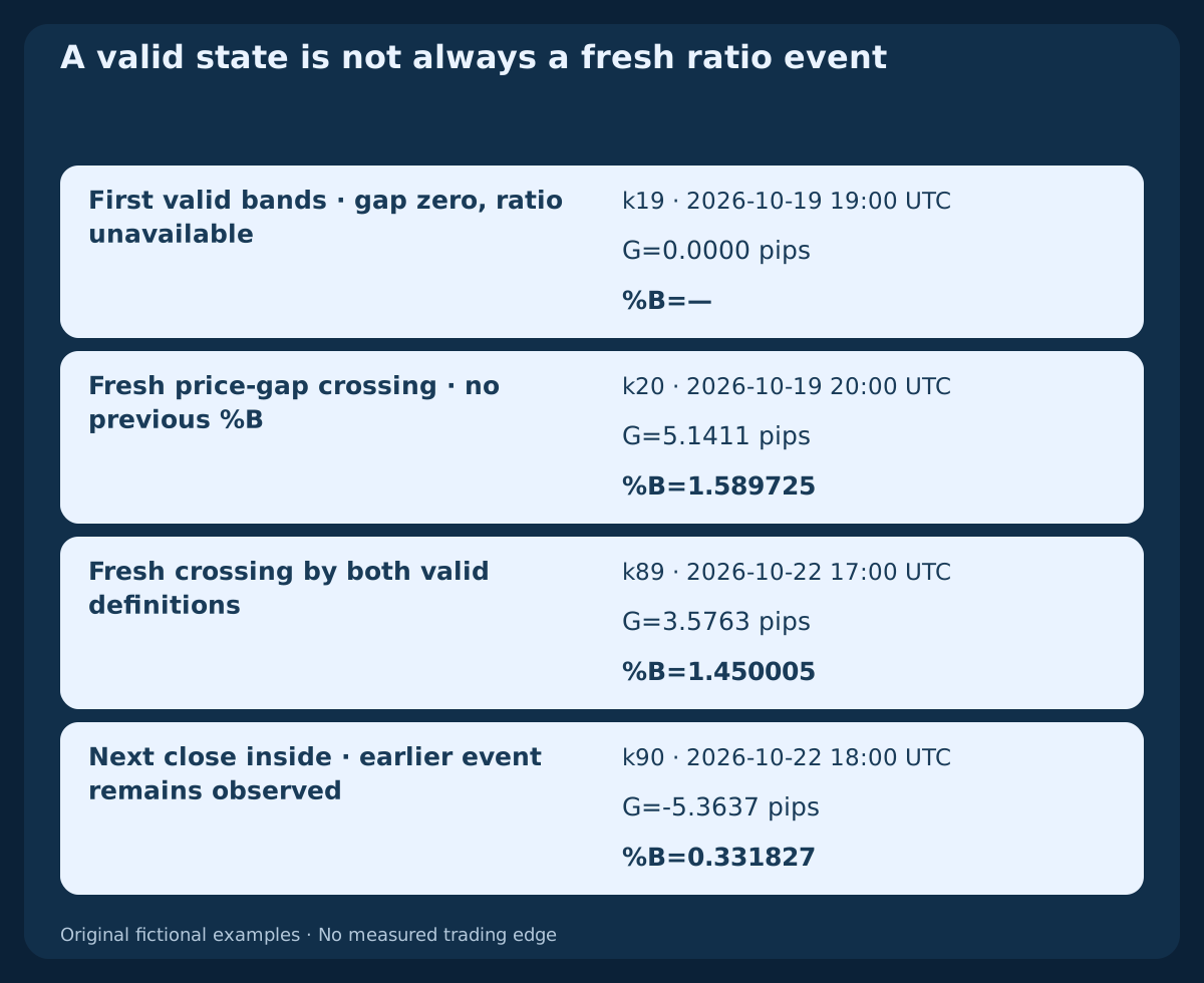
For an upper close, define G(k)=C(k)−U(k). One fresh strict crossing is G(k−1)≤0 AND G(k)>0. Each observation uses its own contemporaneous band. Equality now is not a strict outside close; remaining above is a state. Comparing price with a frozen earlier band is a different rule that must be named.
When both band widths are positive, the corresponding location event is %B(k−1)≤1 AND %B(k)>1. At k19, G is valid zero but %B is unavailable. Thus k20 is a valid raw-gap crossing with no valid previous %B for its normalized counterpart. Both event definitions qualify at k89; k90 is strictly inside. None of these observations alone authorizes an order or retry.
8. Explain window expiry before interpreting contraction
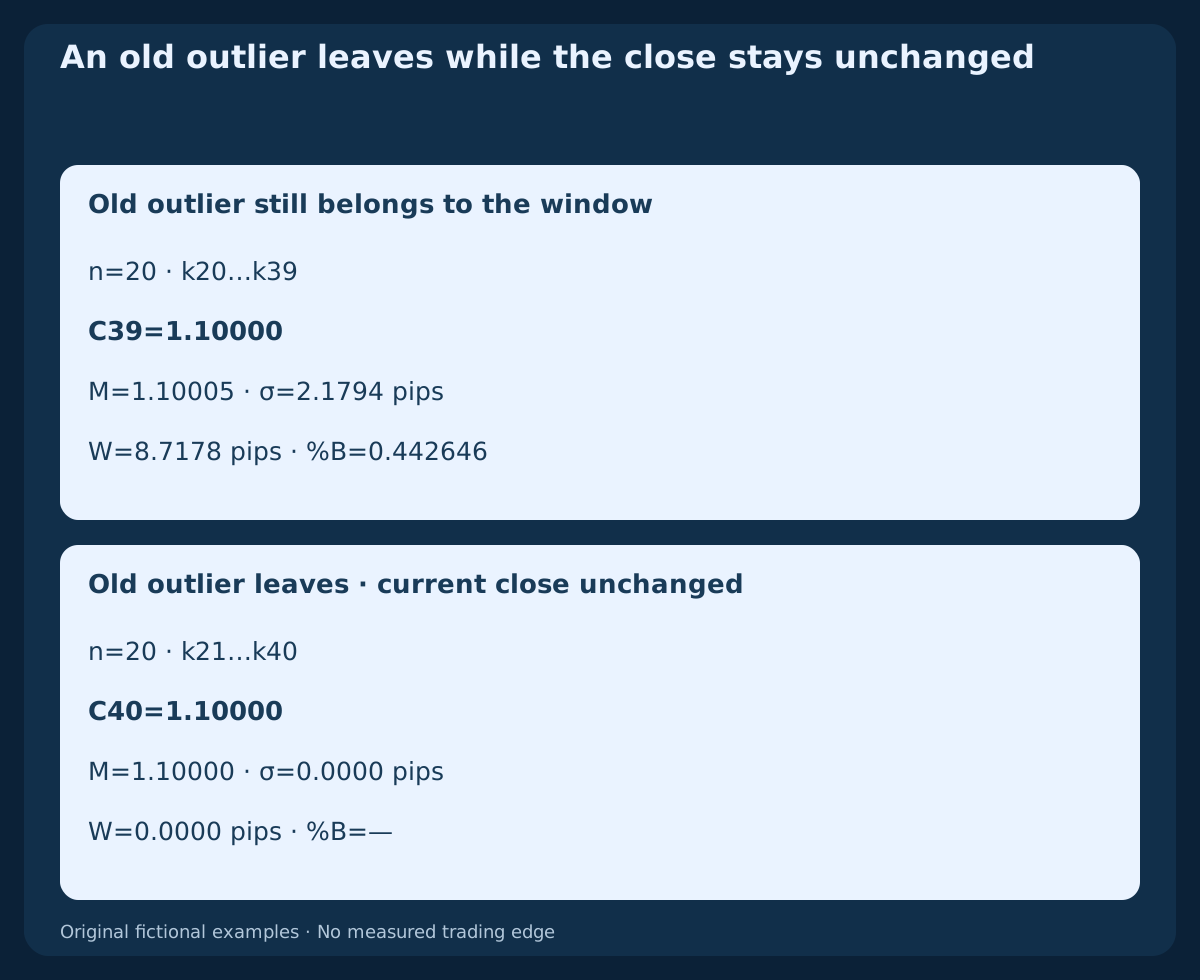
Compare k39 with k40: C39=C40=1.10000. The isolated outlier at k20 belongs to the window k20…k39, then leaves k21…k40. The latter is completely flat. Bands collapse although the latest close has not moved.
This finite-window change does not show a future trading opportunity, a reversal or when activity will return. Price-level standard deviation can also increase during orderly drift. It measures dispersion of closes around their mean; it does not measure intrabar high-low range or establish that current price movement is accelerating.
9. Read range and trend context without automatic fading
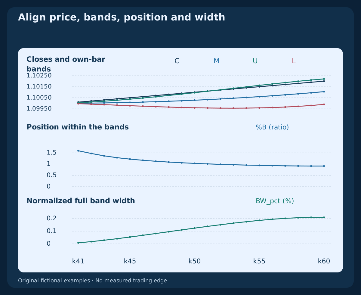
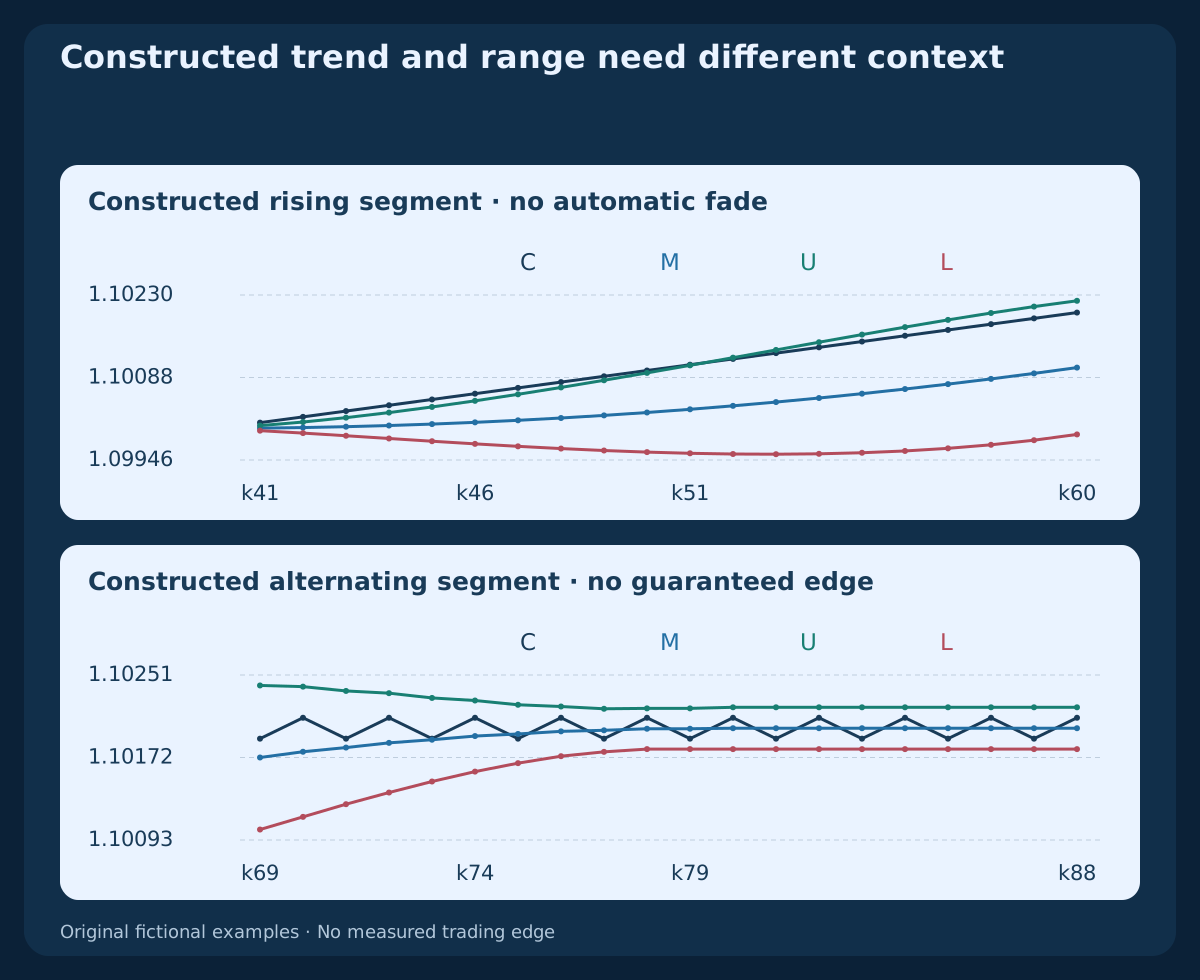
The constructed rise k41–k60 and alternating segment k69–k88 answer different visual questions. In the rise, k41–k51 close above their own upper bands, then the price continues rising while its relative location moves inside. Repeated upper observations are compatible with continuation; they do not repeatedly renew a fresh entry.
The alternating segment is deliberately built, not a regime classifier validated on broker history. Its early rolling windows still contain closes from the preceding rise. A narrow or apparently horizontal envelope does not guarantee that its next edge will hold. Define context from information available before the proposed decision, rather than naming a successful range or trend after seeing the outcome.
10. Define narrow relative to earlier valid widths
An illustrative strict comparison is BW_pct(k)<min(BW_pct(k−10),…,BW_pct(k−1)). The current value is excluded from the reference set; all 10 previous values and the current value must be available. Equality with the earlier minimum is not a new strict low. A persistent low state is also not a fresh record at every bar.
This short teaching comparison is not an implementation of a 125-period Squeeze convention. At k40, width is a new relative low but %B remains unavailable. A width condition cannot repair the missing ratio. Contraction specifies neither breakout direction nor timing, and a later expansion does not retroactively make an earlier observation tradable.
11. Change window length and multiplier separately
The main CSV compares 20 / 2 with 10 / 2 and 20 / 3. The shorter model first exists at k9; all three have complete windows over k19–k90. Compare location ratios only where each required band width is positive. Changing length changes both the mean and dispersion. Changing only the multiplier retains those values and stretches the same envelope.
For three rather than two deviations, full width and normalized width increase by 1.5; for nonzero width, %B_3=0.5+(%B_2−0.5)×2/3. This algebra does not identify an optimal setting. Compare complete rules on the same valid sample, with execution and exits held consistent, before attributing benefit to fewer or later observations.
12. Keep the MT4 buffer clock separate from display offset
A reference call is iBands("EURUSD",PERIOD_H1,20,2,0,PRICE_CLOSE,MODE_MAIN,1). Request MODE_UPPER and MODE_LOWER with the same inputs. Here bands_shift=0 keeps the display undisplaced, while shift=1 requests the latest completed bar after the next bar and data are available.
A request at shift=0 reads a forming bar and can change intrabar. Display displacement is a separate setting and supplies no future information. Verify history availability and actual broker symbols; do not treat an error or missing buffer as a valid flat window. Reconcile applied price, timestamps and data gaps. The fixture is a declared calculation, not terminal-parity certification.
13. Separate the observation from an executable BUY budget
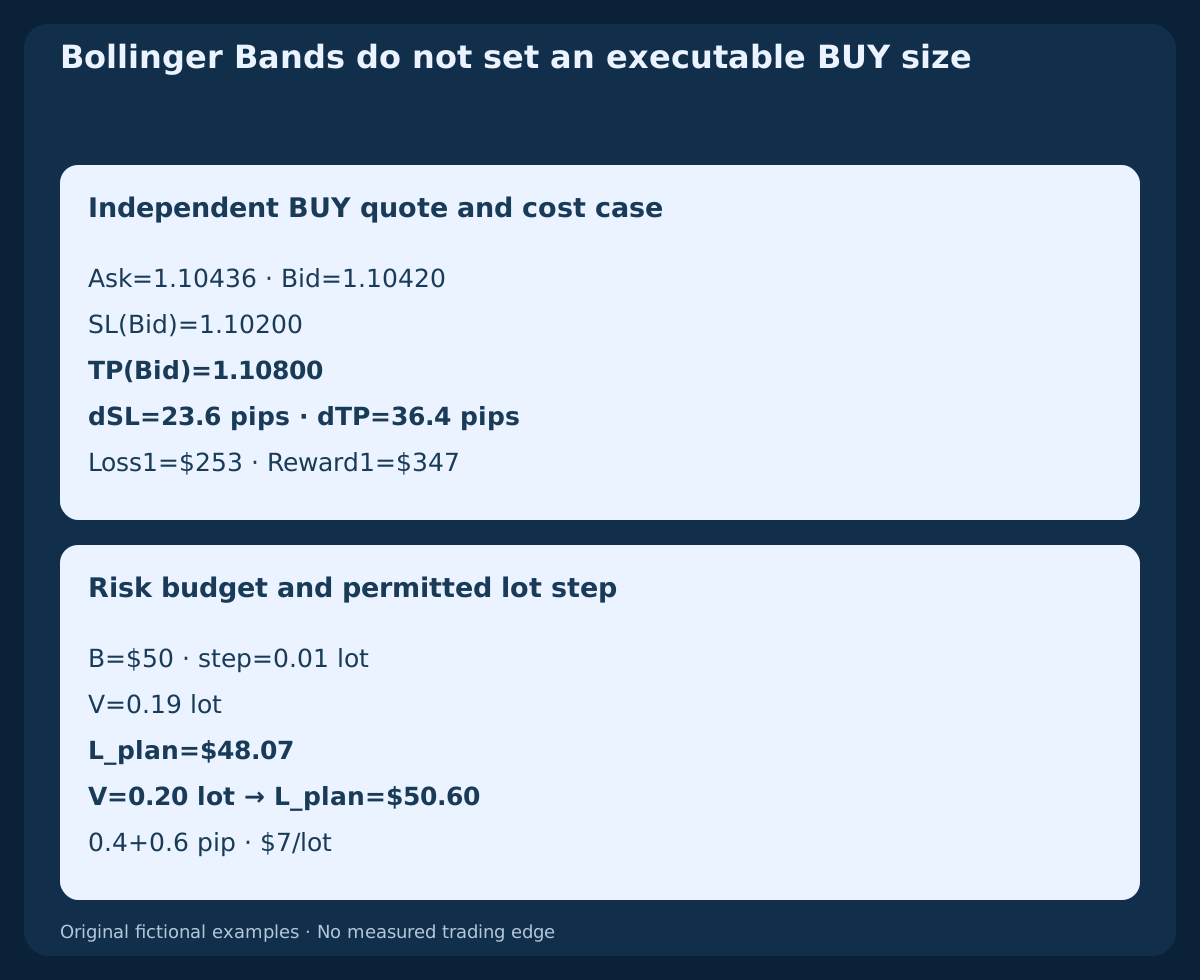
Consider an independent fictional BUY calculation: Ask=1.10436, Bid=1.10420, SL(Bid)=1.10200 and TP(Bid)=1.10800. A long enters at Ask and its protections use Bid. The stop distance is 23.6 pips and target distance 36.4 pips. This is not a trade from the close-only fixture, which has no historical Ask or fill path.
Assume $10/pip/lot, round-trip commission $7/lot, separate adverse reserves a_entry=0.4 pip; a_exit=0.6 pip and declared zero funding. Then Loss1=(23.6+1)×10+7=$253 and Reward1=(36.4−1)×10−7=$347. A $50 budget with a 0.01-lot step allows 0.19 lot and planned loss $48.07; 0.20 lot would risk $50.60. The distances already use the correct quote sides: do not add spread again. Verify actual tariffs, margin and fills; the planned reserve does not cap actual loss.
14. Evaluate a complete rule rather than a band shape
Before testing, specify the price source, population convention, band displacement, ratio units, availability and exact event. Name any frozen reference, pre-event context and condition expiry. Add order timing, entry, cancellation, stop, target, size, exit and uncertain-order handling. A completed signal is not a same-close fill guarantee.
Compare a baseline with and without each extra filter under identical execution assumptions. Bands, %B and BandWidth share the same prices; agreement does not make them independent evidence. Reserve evaluation data, log parameter trials and report costs, sample size, drawdown and uncertainty. Attractive selected examples cannot demonstrate a prospective trading edge.
15. Reproduce the original fixture and its limits
The main CSV contains 91 fictional EURUSD H1 Bid closes from 2026-10-19 00:00 UTC, beginning at 1.10000. It includes the default, both parameter comparisons and a separately named sample-dispersion comparison. The second CSV contains independent fixed-band boundary geometries, including a zero-width case, not observations from the close history.
Means and variances use exact rational arithmetic; square roots and derived values use eighty-digit Decimal calculations before rounded export. Table prices are rounded to five decimals, whereas event decisions use full precision. There are no observed broker candles, highs/lows, intrabar paths, historical Ask values or orders. No historical backtest, measured accuracy or profitable setting is reported.
Download 91 fictional H1 closes and Bollinger parameter comparisons (CSV)
Download six independent %B boundary and zero-width cases (CSV)
| Index | UTC close | Bid close | M20 | U20x2 | L20x2 | %B (ratio) | BW_pct (%) |
|---|---|---|---|---|---|---|---|
| 19 | 2026-10-19 19:00 UTC | 1.10000 | 1.10000 | 1.10000 | 1.10000 | — | 0.0000 |
| 20 | 2026-10-19 20:00 UTC | 1.10100 | 1.10005 | 1.10049 | 1.09961 | 1.5897 | 0.0792 |
| 39 | 2026-10-20 15:00 UTC | 1.10000 | 1.10005 | 1.10049 | 1.09961 | 0.4426 | 0.0792 |
| 40 | 2026-10-20 16:00 UTC | 1.10000 | 1.10000 | 1.10000 | 1.10000 | — | 0.0000 |
| 60 | 2026-10-21 12:00 UTC | 1.10200 | 1.10105 | 1.10220 | 1.09990 | 0.9119 | 0.2095 |
| 88 | 2026-10-22 16:00 UTC | 1.10210 | 1.10200 | 1.10220 | 1.10180 | 0.7500 | 0.0363 |
| 89 | 2026-10-22 17:00 UTC | 1.10280 | 1.10204 | 1.10244 | 1.10165 | 1.4500 | 0.0721 |
| 90 | 2026-10-22 18:00 UTC | 1.10190 | 1.10204 | 1.10244 | 1.10163 | 0.3318 | 0.0728 |
16. Keep a practical reading checklist
Identify the instrument, feed, bar length, applied price, window, multiplier, variance divisor, displacement, units and available history. Then name what you observed: relative position, width, a continued state, a fresh crossing or an independently defined context. Missing required data remain a limitation rather than an invented value.
Only a separate complete trading specification can connect that reading with an entry, protection, size and exit. The related combination and strategy articles use their own decision rules. Keep the baseline fixed when assessing extra confirmation, delay and costs instead of assuming an additional indicator improves the method.
Frequently asked questions
What do Bollinger Bands 20/2 mean?
Twenty bars for the simple average and population dispersion, with two standard deviations on each side. On H1 these are bars, not days. Also specify price source and display offset; defaults do not establish profitability.
Does touching a band mean buy or sell?
No. A touch describes relative location. Prices can continue near or beyond a band. Entry, invalidation, protection, size and exit require a separate complete rule.
Can %B be below zero or above one?
Yes. On the ratio scale, zero is the lower band and one the upper. A value 1.25 means one quarter of the full band width above the upper band. Zero band width makes this reference ratio unavailable.
Why do BandWidth displays differ by one hundred?
Raw width divided by the middle is a ratio; multiplying by one hundred expresses the same value as percent. Inspect the formula and units. A historical-range normalization called %BandWidth can be a different indicator.
Are closed buffers the same as shifted bands?
No. Buffer shift selects an observation, while display displacement changes chart alignment. This guide uses zero displacement and the latest completed observation after data are available. Neither setting supplies future prices.
Do two standard deviations guarantee 95% containment?
No. The construction alone establishes no fixed future probability. Market distributions, rolling dependence and context matter. These fictional examples do not estimate coverage or trading performance.
Sources and research notes
Primary sources support traditional construction, inputs, display timing and width/position definitions. The close history, boundary geometries, parameter comparisons, availability policy and BUY arithmetic are original educational constructions. They do not certify broker/platform parity or trading performance.
- MetaTrader 4: Bollinger Bands and population dispersion
- John Bollinger: BandWidth and %BandWidth definitions
Educational Bollinger guide. Fictional closes, independent assumed band geometries and a separate cost case; no broker orders, historical backtest or measured profitability.